


 – Dia 2")
 and Biotechnology")


AMAZON
Breaking down the famous style transfer algorithm for beginners !
https://medium.com/media/b4dca21b5f98a315f9e595b6889abe71/href
Trending AI Articles:
In this tutorial, I am going to talk about Neural Style Transfer, a technique pioneered in 2015, that transfers the style of a painting to an existing photography, using neural networks i.e. Convolutional Neural Networks. The original paper is written by Leon A. Gatys, Alexander S. Ecker, and Matthias Bethge.
The code used for this article can be forked from this repository.
In my honest opinion, this is one of the coolest machine learning applications. It has percolated into mobile applications as well. One such example is of Prisma. A mobile application where in you can use styles of paintings to apply over your photograph in real time.
Looks cool and exciting right? Let’s dive in and implement our own style transfer algorithm.
Note: Before reading on further, it is highly recommended to read the original paper once or read the sections in parallel, so as to ensure you understand the article as well as the paper.
Components
- Introduction and Intuition
- Content Representation & Style Representation
- Content Reconstruction & Style Reconstruction
- Implementing Style Transfer in Keras
Introduction & Intuition
The style transfer algorithm draws its root from the family of texture generation algorithms. The key idea is to adopt the style of one image while conserving the content of the other. This can be formulated as an optimisation problem. We can define a loss function around our objective and minimise the loss.
For the ones, who love mathematics: this can be represented as
loss = distance(style(reference_image)-style(generated_image)) + distance(content(original_image)-content(generated_image))
Let’s break it down bit by bit…
distance is a norm function such as the L2 norm
content is a function that takes an image and computes a representation of its content
style is a function that takes an image and computes a representation of its style
So, plugging in all of these: we can see that minimising the loss causes style(reference_image) to be close to style(generated_image) and similarly content(original_image) to be close to content(generated_image). This is what was our objective, right ?
Content Representation and Style Representation
Let us begin by getting a clear understanding of what do we really mean by content and style ?
Content is the higher-level macro structure of the image.
Style refers to the textures, colours and visual patterns in the image.
Assuming you understand how CNNs work: they will identify local features of the image at the initial layers. The deeper we dive into the network, more higher level content is captured as opposed to just pixel values.
Each layer aims to learn a different aspect of the image content.
It is reasonable to assume that two images with similar content should have similar feature maps at each layer.
We will say x matches the content of p at layer l, if their feature responses at layer l of the network are the same.
Deriving the style loss is a little tricky !
The feature responses of an image a at layer l encode the content, however to determine style we are less interested in any individual feature of our image but rather how they all relate to each other.
The style consists of the correlations between the different feature responses.
We will say x matches the style of a at layer l, if the correlations between their feature maps at layer l of the network are the same.
We will utilise something known as Gram Matrices for deriving the style representation.
We pick out two of these different feature columns (e.g. the pink and the blue dimensional vectors), then, we compute the outer product between them.
As a result, it will give us a CxC matrix that has information about which features in that feature map tend to activate together at those two specific spatial positions.
We repeat the same procedure with all different pairs of feature vectors from all points in the HxW grid and averaged them all out to throw away all spatial information that was in this feature volume.
Content Reconstruction and Style Reconstruction
Our objective here is to get only the content of the input image without texture or style and it can be done by getting the CNN layer that stores all raw activations that correspond only to the content of the image.
It is better to get a higher layer, because in CNN, first layers are quite similar to the original image.
However, as we move up to higher layers, we start to throw away much information about the raw pixel values and keep only semantic concepts.
Note the size and complexity of local image structures from the input image increases along the hierarchy.
Heuristically, the higher layers learn more complex features than lower layers, and produce a more detailed style representation
If you have made this far…Well congratulations to you ! You have understood the core machinery of the style transfer algorithm.
Moving onto the most exciting part now: IMPLEMENTATION !
Implementing Style Transfer in Keras
Style transfer can be implemented using any pre-trained CNN. This tutorial uses the VGG19 network, which is a simple variant of VGG16 network with three more convolutional layers.
General flow of the program
- We will setup a network that can compute the VGG19 layer activations for the content image, style image and the generated image simultaneously.
- Define the loss functions using the layer activations of the images and further minimising them in order to achieve style transfer.
- Setting up a gradient-descent process to minimise these loss functions.
Setting up the environment
Kindly follow these installation notes to setup the environment. You will up and running in no time !
Defining the initial variables
We will begin by defining the paths for the style reference image and the target image. Style transfer can be difficult to achieve if the images are of varying size. Therefore, we will resize them all to have same height.
https://medium.com/media/e8e617e3f3fad8a18af921e7cb121863/href
Image pre-processing and de-processing
https://medium.com/media/f8554b381be6cb587ad305cf8dd8a714/href
Loading the pre-trained network
We will now setup the VGG19 network to receive a batch of three images as input: a style-reference image, the target image and a placeholder that will contain the generated image.
The style-reference image and target images are static and thus defined using K.constant
On the other hand, the generated image will change over time. Hence, a placeholder is used to store the same.
https://medium.com/media/6ec14298c939b8f3e6141d8f6e2a0d2b/href
Defining the loss functions
Content Loss : It is the squared-error loss between the feature representation of the original image and the feature representation of the generated image
https://medium.com/media/75be0658e5f25cb1a36f7558618fa191/href
Computing Gram Matrices : We reshape the CxHxW tensor of features to C times HxW, then we compute that times its own transpose.
We can also use co-variance matrices but it’s more expensive to compute.
Style Loss: First, we minimise the mean-squared distance between the style representation (gram matrix) of the style image and the style representation of the output image in one layer l.
https://medium.com/media/7c997016d2c8b2727bfd5d8997376076/href
Total Variation Loss is the regularisation loss between the content and style images. It avoids overly pixelated results and encourages spatial continuity in the generated image.
The constants a and b dictate how much preference we give to content matching vs style matching.
https://medium.com/media/ec2e12022bfff499763e94034a9664c4/href
Defining the final loss
The loss we will be minimising is the weighted average of these three losses.
To compute the content loss, we use only one upper layer — block5_conv2 layer.
The style loss, on the other hand uses a list of layers that resides in both the high and low levels of the network.
https://medium.com/media/b6e586d09a16277a649771c90ca7e31b/href
Gradient descent process
We will be setting up a class named Evaluator that computes the loss functions and the gradients at once. It will return the loss value when called the first time and caches the gradients for the next call.
https://medium.com/media/c62be4467b490bb5d812d8e7acfb52eb/href
Style transfer loop
We will use SciPy’s L-BFGS algorithm to perform the optimization. It can only be applied to flat vectors. Hence, we will be flattening the image before passing it across.
https://medium.com/media/ebf170580e26652035bc5bdeee53f1f1/href
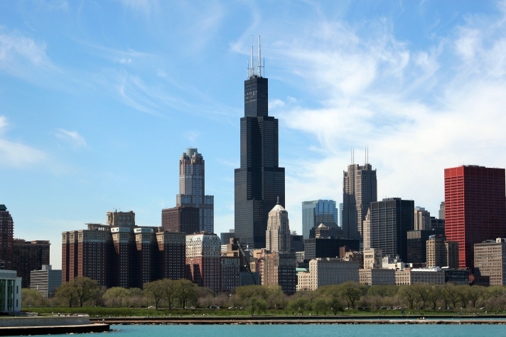
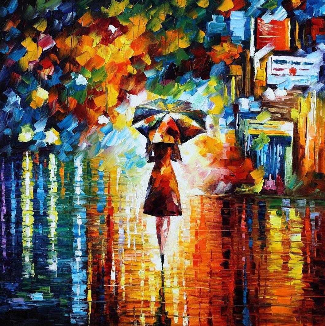
Running this code with the Chicago city photograph as the content image and the Rain Princess as the style image will fetch you this result.
Congratulations !!! You have implemented the style transfer algorithm successfully !!!
https://medium.com/media/d870c8276e8c4b2b1048d97baec1c4e5/href
Hope you learned something by this article.
References
cs231n: Visualizing and Understanding — Stanford University School of Engineering
Don’t forget to give us your 👏 !
https://medium.com/media/c43026df6fee7cdb1aab8aaf916125ea/href
Utilising CNNs to transform your model into a budding artist was originally published in Becoming Human: Artificial Intelligence Magazine on Medium, where people are continuing the conversation by highlighting and responding to this story.